Source data from multiple sheets
If your data lives across multiple Google Sheets or multiple tabs, Portant only reads from one tab. To work around this, combine the data into a single tab using IMPORTRANGE or ARRAYFORMULA, then point Portant at that combined tab.
This page covers how to set up that combined tab, how to write formulas that don't break on empty rows, and an alternative tool for syncing data across sheets.
Combine data from multiple sheets into one tab
Make a new tab (in an existing spreadsheet, or in a new one) that will be the single source for your workflow. Then pull in the data you need.
To pull data from another spreadsheet, use IMPORTRANGE:

- For a single cell:
=IMPORTRANGE("https://docs.google.com/spreadsheets/d/abcd123abcd123", "sheet1!A1") - For a range:
=IMPORTRANGE("https://docs.google.com/spreadsheets/d/abcd123abcd123", "sheet1!A1:C10")
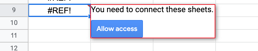
The first time you reference a spreadsheet, Google will ask you to allow access. You only have to do this once per source spreadsheet.
To pull data from another tab in the same spreadsheet, use ARRAYFORMULA:
=ARRAYFORMULA(Sheet1!A:C)
Once your combined tab is populated, point your Portant workflow at it.
Stop empty rows from showing errors or zeros
When you copy a formula down a column, the empty rows often return #REF!, #N/A, or 0. Portant treats these as populated rows, which can break auto-create. Wrap your formulas so they return a blank for empty inputs.
To handle errors, use IFERROR:
=IFERROR(A2*100, "")
To handle blanks, use IF:
=IF(A1="", "", A1*100)
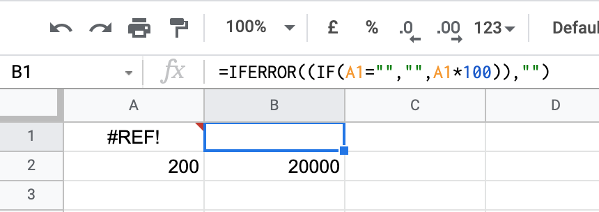
You can combine both for the most defensive version:
=IFERROR(IF(A1="", "", A1*100), "")
Use Coefficient to sync data across sheets
If formula juggling isn't your thing, Coefficient is a Google Sheets add-on that imports data from other sheets, CRMs, and accounting tools, and refreshes it on a schedule.
To get started, sign up for Coefficient, install the add-on, and open the Coefficient pane in your sheet.
Click Import Data:

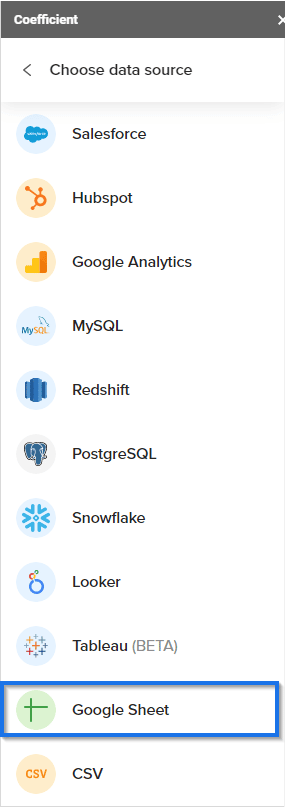
Select Google Sheet:
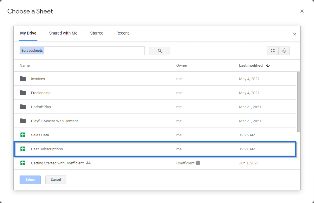
Pick the source sheet from your Google Drive and click Select:
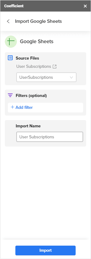
Coefficient reads the columns and shows you an import panel where you can filter the data:
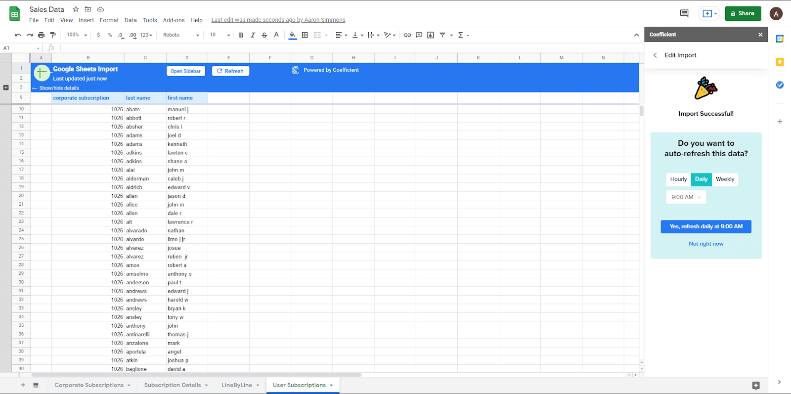
Click Import and the data appears in your sheet.
To keep the data fresh, set up an auto-refresh schedule:
Compared to IMPORTRANGE, Coefficient handles filters during import and adapts when the source data shifts, so you don't have to redefine ranges manually.
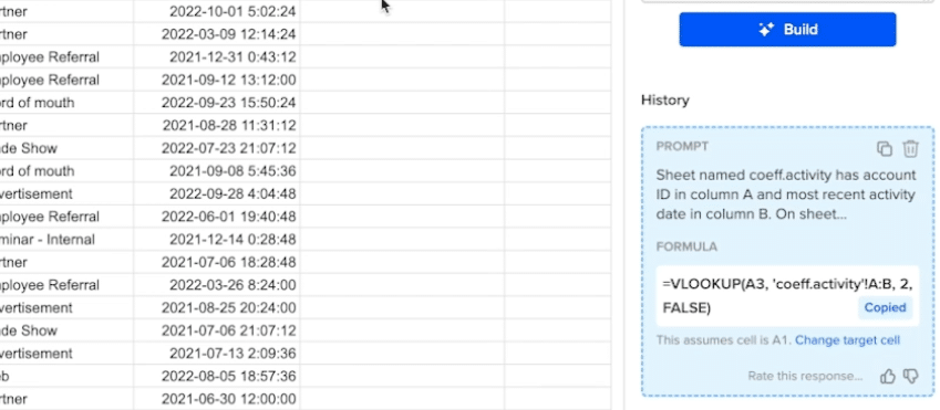
If you want to build reports off the combined data, Coefficient's GPT Copilot can write formulas, pivots and charts from plain text instructions:

It returns a working formula: