Add formula fields to a Google Forms workflow
Sometimes you want to insert content based on a form answer without asking the respondent for it directly. For example, if someone picks an office location, you might want to auto-fill the address, phone number and email for that office.
Most of the time you can do this with tag formulas or tag if statements. If those don't fit, this page shows how to add formula columns to a Google Forms response sheet and use that sheet as your workflow source.
Set up a workflow on the response sheet
In your Google Form, click the Responses tab and then the Google Sheets icon to create or link a response sheet:

You can either create a new spreadsheet or add a tab to an existing one. From now on, every form submission will land as a row in this sheet.
In Portant, create a new workflow and pick that sheet as the source. With auto-create on, Portant checks the sheet every couple of minutes and runs the workflow on any new rows.
Add formula columns to the response sheet
So far this is just a Google Sheets workflow. The trick is adding formula columns that calculate extra values based on the form answers. There are two ways to do it.
Option 1: array formula in row 2 of the response sheet
Click the cell in row 2, just to the right of your last form-response column. Type =ARRAYFORMULA(...) with your formula inside. The array formula will fill down the column as new responses arrive.
=ARRAYFORMULA(A2:A*2)
This doubles the value in column A for every row.
You can also use an IF statement to insert content conditionally. For example, this returns "This value is Yes" whenever column A is "Yes", and a blank otherwise:
=ARRAYFORMULA(IF(A2:A="Yes", "This value is Yes", ""))
Press Enter and the formula will apply to every row, including new responses as they come in.
Option 2: array formula in a new tab
If you'd rather keep the response sheet untouched, or if your formula doesn't play well with arrays, copy the response data into a new tab and add your formulas there.
We recommend an array formula to mirror the responses:
=ARRAYFORMULA(Sheet1!A:X)
Where A is the first response column and X is the last. Then add your extra formula columns to the right of the mirrored data. Point Portant at this new tab as the source.
Stop empty rows from showing errors or zeros
When a formula is filled down a column, the empty rows often return #REF!, #N/A, or 0. Portant treats those as populated, which can break auto-create. Wrap your formulas so they return blank for empty inputs.
To handle errors, use IFERROR:
=IFERROR(A2*100, "")
To handle blanks, use IF:
=IF(A1="", "", A1*100)
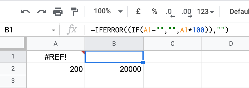
Or combine both for the most defensive version:
=IFERROR(IF(A1="", "", A1*100), "")